Obsolete by the Great Simplification … yet still useful for heuristics
The central result of the cited articles from Stephen Hawking(1) and David Malament(2) is the proof that the path-topology, and only the path-topology, of space-time defines the time-like curves and viceversa, i.e. the time-like curves define uniquely the topology, where in turn the metric Tensor g may be reconstructed up to a conformal factor –in case of Lorentzian Manifolds- from the underlying topology.
This result is transcendental in our context, as hence time-like curves can be defined using only means of set-topology, that is without the heavy baggage of Pseudo-Riemann Manifolds etc. etc. and their implicit baggage of Real Analysis, Linear Algebra, Infinity anywhere etc. etc.
This stripped-down model of space-time can be extended without sacrificing its essential mathematical content to finite and countable models, something that can’t be done, at least no so easy, while –Einstein never said we had to- sticking to Lorentzian Manifolds supposedly as only feasible mathematical model underneath GRT.
… and we are almost there. Let’s see what still was missing in Part II:

Here we’ve got our already standard grid twice: once as-is, once flipped along the magenta axis of arrows, while the green arrows invert their direction. This transformation in blue coordinates corresponds to interchange the space- and the time-coordinate, a symmetry with profound physical interpretation. However –remember the coordinates by now have no meaning by themselves- the two grids are until now topologically identical: there is a 1-to-1 correspondence of boxes and connectors.
This means that only with this topology, the one defined until now, there is no way to preserve orientation or more general identify time-like curves only by means of topology. Actually, the picture already hints what to do: the time-arrow changed position (right side<>below), such that if we include the time arrow as additional connectors into the grid, we might be done.

We marked with a smiley two boxes, which before adding the additional connectors were topologically symmetric under the interchange of time and space and now are not. Noteworthy, the additional connectors were already present at some earlier stage of the development of net-theory and had their own name observables, as we will see –maybe- in a later post by no means a name by chance. And by then at least I knew already, that they are essential to define orientation respectively natural orders, i.e orders completely defined by their topology. So welcome back.
This is the content of
Axiom 7 Loops

Axiom 7.1 defines objects similar to the standard one-dimensional sphere, yet without relying on other concepts than our Axioms defined so far. The first line expresses that it should have just one dimension by requiring any 4 distinct points to be related. The second that it should comply with all Axioms defined so far, which as we’ve seen before among other orders all it points as on a circle. The third line requires double-connectivity, exactly what makes the difference between a Circle and the Real Line before one-point-compactification.
The unit-circle is one possible representation of S but likewise any other simple, closed curve i.e Jordan-Curve in the 2-plane or any homeomorphic image of the S, as from the point of view of Q they all are identical.
Axiom 7.2 defines a subset of the set of mappings from S to Q, requiring that the mapping produces an image –a curve- with at least 4 elements –remember 4 points on a circle, that’s where we started- and is an continuous mapping in the respective topologies. In traditional settings –everything at least a Hausdorff-Space- one would continue -defining paths and curves- requiring an injective mapping, we ask only –in the second line- for some form of monotony, which actually preserves orientation and excludes overcrossings. Requiring an injective mapping would carry a Hausdorff-property over to Q, which means no finite and only quite weird countable models, against all our intention. The last part of Axiom 7.2 defines a class of subsets, those that are image of some closed path, it may be understood as a generalization of the concept of Jordan-Curves. Please note that J-Curves are always closed and that they may change direction while going through Q.
Axiom 7.3-4 introduces the concept of J-connected points of a set –they may be connect by a connected piece of a J-curve, completely in the set- and J-convex sets, i.e. sets where every two points may be J-connected.
Before continuing, let’s get back to our augmented model-grid, see how Jordan-Curves may look like and if we got now sufficient to tell time- and space-axis apart using only topological means.

First some Jordan-Curves (remember: connectors are noted by their adjacent boxes):
blue {(0,0), {(0,0),(-1,1)}, (-1,1), {(-1,1),(0,2)}, (0,2), {(0,2),(1,1)}, (1,1),{(1,1),(0,0)}}
red {(0,0), {(0,0),(-1,0)}, (-1,0), {(-1,0),(0,-1)}, (0,-1), {(0,-1),(0,0)}
We show two candidates for cones at (0,0) a black cone set, that would correspond to the time-axis and a light blue one, that might correspond to a space-axis. Finally we shadowed the area, the smallest where the asymmetry between time and space makes itself manifest.
We observe in this area: both halves of both cones are J-connected, i.e. there is a J-Curve inside that connects any two points. Going from half to half of a cone, every inner connecting J-Curve contains (0,0) and at least one additional point, that is not part of the respective cones. There is however a difference: any J-curve in one of the black cone-halves contains at least one third element (0,2) , (0,-2) that connects directly to the center point (0,0), while this element does not exist in the light blue one, a connection established precisely by the additional connectors we added.
Actually with these observations we’re done already, if we put them into a mathematical language in a way that extends to all our structures, avoiding pitfalls like for instances that already in the 2+1 Grid (2 space-, 1 time-coordinate), there are no longer halves of the space-cone.
Axiom 7.5-6 introduces some necessary technalities, first locally connected sets then, as not all our points are closed, what may be called a saturated open set, i.e. open sets that with a neighborhood of a point contain also the point itself, third the set of open points –if there are- and finally the closed hull of a point, meaningful if it’s a open point.
Now the core of the Axiom itself:
Axiom 7.7

Lets check against our model grid, if the Axiom 7.7 does indeed would we like that it does (and that way go through it line by line).
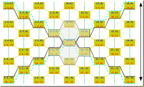
For the beginning, let’s just note that here connectors represent no problem, as they have just one box at entry, one box at exit, so most of the conditions are void.
Now boxes:
The first line of Axiom 7.7 says that there should be an open set that includes the hull of the box as a sort of limiting our scope to some open neighborhood. The gray shadowed area above may be such a neighborhood.
The second line asks that all open sets, which include the hull and are contained in our starting neighborhood, shall satisfy some conditions, i.e. once found, the axiom somehow propagates from outer to inner.
The third line asks that each of these contained open-sets should have a decomposition into 2 new open sets (sets with <- and –> on top, they will be our the local cones). Their join with the point-set {x} shall be the open-set on study, their meet contain only open points.
In our example,
{(0,0), {(0,0},(-1,1)}, (-1,1), {(-1,1),(0,2)}, (0,2), {(0,2),(1,1)}, (1,1), {(1,1),(0,0)},{(0,0),(0,2)}} is one of the candidates, it’s below dual the other.
Now the conditions, symmetric for both halves, the partition shall satisfy:
 For every pair of distinct points y, z in the same halve and any neighborhood of the hull of the point x under study, there shall be always a J-Curve that runs within the saturated pre- (respectively post-) cone. It shall contain all three points x,y,z and at least one additional point in that neighborhood. This way we formalize the above idea of directly connected. A rapid look on the picture shows that this is indeed the case.
Be aware that the set of boxes {(0,0), (-1,1), (0,2), (1,1), (1,-1), (0,-2), (-1,-1)} is the smallest possible open neighborhood of the hull for x and the above introduced candidates for cones are the smallest possible saturated open sets to cover these boxes, then it’s easy to see that again our picture fits into the axiom: every closed J-Curve contains at least three boxes from the neighborhood of the hull .… and it’s likewise relatively easy to see why the space-cones do not fit.
The Lemma A.17

shows that, as intended, curves that connect points in different cones, run trough the tip x of the cones and contain at least one outside element.
We omit for the moment additional technalities, like that each cone shall be J-convex and their intersection shall consist only of open points, which however will be important in later contexts and posts.
We note without proof here –but there will be in a later post- already one fundamental result: the Q-Loops define Q and viceversa, actually not such a big surprise looking at homotopy-theory and it’s results.
This ends our presentation of Axiom 7.
1 S. W. Hawking A.R. King and P. J. McCarthy, A new topology for curved space-time which incorporates the causal, differential and conformal structures Journal of Mathematical Physics Vol. 17, No 2, February 1976
2 D. Malament, The class of continuous timelike curves determines the topology of spacetime Journal of Mathematical Physics, July 1977, Volume 18, Issue 7, pp. 1399-1404


 Posts
Posts

